6 Step Optimization of GeMMs in CUDA
I aim to take a naive implementation of single-precision (FP32) General Matrix Multiplication (GeMM) and optimize it so its computations can be parallelized effectively on GPUs with CUDA C/C++.
With this post, I aim to take a naive implementation of single-precision (FP32) General Matrix Multiplication (GeMM) and optimize it so its computations can be parallelized effectively on GPUs with CUDA C/C++. Alongside this article, I also have Github implementation of these methods. While here I only showcase the final kernels with their methods, my GitHub repository includes more detailed information that will assist you in recreating this work.
For this article, I will assume you are familiar with GPU architecture and systems, parallel computing, GeMM, and CUDA C/C++.
[Sorry about the code! Ghost doesn't have a great way to show code. Please check out my github or medium article instead]
Let’s get started!
Understanding the Algorithm
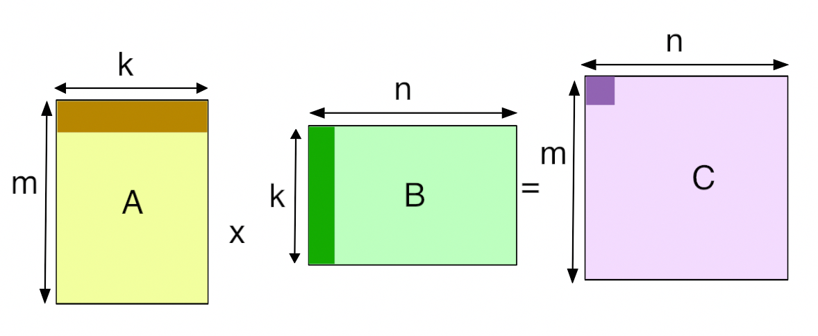
The algorithm is a very simple, “Hello-world”-equivalent problem in the linear algebra world. General Matrix Multiplications (GeMM) simply take two matrices A and B and multiply them together. Matrix multiplication is a bit different from scalar multiplication, however. Let’s assume Matrix A is an m x n matrix and Matrix B is an n x k matrix. In order to multiply A with B (order matters), we need to first need to take the dot product of rows of A with cols of B , and then add them together. Then it is stored in another matrix, Matrix C, which has dimensions m x k.


But we should all already know this.
There is one more thing to keep in mind — when you look up GeMM or SGeMM (Single Precision GeMM), you would often find the equation C = (alpha*(dot_prod)) + (beta*C). This notation is used to allow for additional scaling factors (α and β) to be used for optimization and specific calculations within linear algebra operations. We don’t have to worry about them here, but it is important to know about.
For our purposes, we will have alpha = 1 and beta = 0. For simplicity, all of out matrices are going to be square matrices, meaning they will have same number of rows and cols making their dimensions to be m x m.
Our Metrics
The point of optimizing an algorithm is to achieve the GPU’s peak performance which hinges on effectively utilizing its compute power and its memory bandwidth. Unoptimized algorithms cause these two factors to act as major bottlenecks for trying to speed our computations and fully utilize out GPUs. To manage and calculate the two, we can calculate them in terms of GFLOPS (Giga Floating Point Operations per Second) and GB/s (Gigabytes per second). We should also calculate the time to see how optimizing compute and memory can speed up the computations exponentially!
In order to optimize these two factors, let’s briefly understand what they are impacted by and what we need to focus on!
- Compute: In order to optimize this, we need to make our computations smarter by making them time efficient. This means looking at runtime complexities, thread allocation/optimization, and how they maybe be broken down at compile time.
- Memory Bandwidth: In order to optimize bandwidth, we need to assess how we can make the data reads and writes faster. We need to understand how and when the data is transferred from global memory (GMEM) to shared memory (SMEM) to registers; it also means we need to understand which part of the data we need to load and when.
With this, let’s get started with a very basic implementation of our algorithm!
GeMM-1 : Naive Implementation
All we aim to do here is simply multiply our two matrices A and B (that are passed into our kernel as d_A and d_B) in a very straightforward manner without any special handling of memory and computation. You make each thread compute one element of the output matrix C (passed in as d_C) by iterating over one row of A and one column of B. This should be a reiteration of what we already know, but coding it in CUDA might make it harder to visualize. Let’s try to simplify the code!
Code Implementation
Understanding this implementation would make future ones a lot easier!
__global__ void naive_mat_mul_kernel(float *d_A, float *d_B, float *d_C,
int C_n_rows, int C_n_cols, int A_n_cols)
{
const int row = blockDim.x * blockIdx.x + threadIdx.x; // row from current thread
const int col = blockDim.y * blockIdx.y + threadIdx.y; // col from current thread
// C[row][col]
// Setting bounds
if (row < C_n_rows && col < C_n_cols){
float value = 0;
// Computing dot product from A_row and B_col
for (int k = 0; k < A_n_cols; k++){
value += d_A[row * A_n_cols + k] * d_B[k * C_n_cols + col];
}
// Resulting C matrix = alpha(dot_prod) + beta[C_mtx]
// alpha = 1 ; beta = 0 ;
d_C[row * C_n_cols + col] = 1 * value + 0 * d_C[row * C_n_cols + col];
}
}
Here, we start with d_A, d_B, and d_C which are just our matrices A, B, and C allocated on device (GPU) instead of host (CPU). C_n_rows , C_n_cols , and A_n_cols are all integer values to understand the size of our matrices.
We start our algorithm by initializing variables row and col based on the thread and block indices, which determine the specific element in the output matrix d_C that each thread will compute, the kernel checks if these indices are within the valid range of matrix d_C's dimensions. If they are, the algorithm initializes a local variable value to zero. This variable will accumulate the sum of products in the dot product calculation between a row of matrix d_A and a column of matrix d_B.
In the loop, value is computed by iterating over the k index which ranges from 0 to A_n_cols, the common dimension between matrices d_A and d_B. For each k, the corresponding elements from d_A and d_B are multiplied together and added to value. Specifically, d_A[row * A_n_cols + k] accesses the element in the rowth row and kth column of d_A, while d_B[k * C_n_cols + col] accesses the element in the kth row and colth column of d_B.
After completing the loop, value contains the dot product of the rowth row of d_A and the colth column of d_B. This result is then stored in d_C at position [row * C_n_cols + col], effectively setting the element at row and col in the output matrix d_C to the computed dot product. The coefficients alpha = 1 and beta = 0 for the line d_C[row * C_n_cols + col] = 1 * value + 0 * d_C[row * C_n_cols + col]; imply a direct assignment with no scaling or addition from the existing value in d_C.
This kernel is executed across all threads in the grid, with each thread computing one element of the resulting matrix d_C, making this a parallel matrix multiplication operation handled via naive method on a GPU.
Results
Let’s look at some results for MxM matrices sized 128, 256, 512, and 1024.
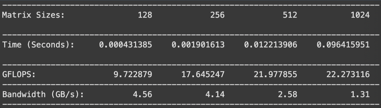
Problems with this method
Larger matrices are going to take longer time and GFLOPs; we can’t make any conclusions there as of now. However, our bandwidth looks awful! Low bandwidth means that the GPU is reading and writing data slow. We can also clearly see that as we scale up our matrices, our approach is suffering from inefficient memory access patterns and excessive GMEM accesses due to cache misses. This leads to high latency and low throughput alongside low bandwidth.
Let’s try to make this a bit better!
GeMM-2 : Coalescing our GeMM
In order to understand coalescing, we need to understand how data is read. When an address space is read, the surrounding address spaces are also loaded on-chip due to caching. With our GeMM-1, we aren’t necessarily accessing address spaces that are next to each other which causes cache misses and makes us travel all the way to global memory to access our value — this is very slow.
This is what coalescing tries to solve. Coalescing improves memory access patterns by trying to have the threads access consecutive memory addresses. This reduces the amount of cache misses because the next element that needs to be accessed would already be on chip and we wouldn’t have to wait for it to be fetched from global memory/DRAM .
Code Implementation
Let’s understand with code!
__global__ void coalesced_mat_mul_kernel(float *d_A, float *d_B, float *d_C,
int C_n_rows, int C_n_cols, int A_n_cols)
{
// Switching the order of row and col for coalescing
const int col = blockDim.x * blockIdx.x + threadIdx.x;
const int row = blockDim.y * blockIdx.y + threadIdx.y;
// everything else stays the same
if (row < C_n_rows && col < C_n_cols){
float value = 0;
// Computing dot product from A_row and B_col
for (int k = 0; k < A_n_cols; k++){
value += d_A[row * A_n_cols + k] * d_B[k * C_n_cols + col];
}
// Resulting C matrix = alpha(dot_prod) + beta[C_mtx]
// alpha = 1 ; beta = 0 ;
d_C[row * C_n_cols + col] = 1 * value + 0 * d_C[row * C_n_cols + col];
}
}
This might seem the dumbest “optimization” ever! All we did is switch the assignment of row with col. How does that change anything at all?
But, as we’ll see with our results, this simple change helps us reduce the number of cache misses by accessing address spaces that are contiguous or right next to each other. Consider multiplying two 4x4 matrices with a 2x2 thread block configuration. In our original GeMM-1, when thread block (0,0) begins execution, the threads would access matrix A and B as follows: thread (0,0) computes element C[0,0] by accessing A’s first row (A[0,0], A[0,1], A[0,2], A[0,3]) and B’s first column (B[0,0], B[1,0], B[2,0], B[3,0]). Meanwhile, thread (0,1) works on C[1,0], accessing A’s second row and B’s first column. This access pattern means our threads are striding through memory with large gaps, particularly when accessing matrix B’s column elements.
With our coalesced version, we’ve reorganized how threads map to the output elements. Now, thread (0,0) still computes C[0,0], but thread (0,1) computes C[0,1] instead. This means that when accessing matrix A, consecutive threads in a warp are reading from the same row of A (A[0,0], A[0,1], A[0,2], A[0,3]), which represents contiguous memory locations. For matrix B, these same threads now access consecutive elements in B’s rows (B[0,0], B[0,1], B[0,2], B[0,3]) rather than striding through columns and always missing.
The actual computation in value += d_A[row * A_n_cols + k] * d_B[k * C_n_cols + col] remains the same, but the memory access pattern has been transformed. When k=0, all threads in the same row of a thread block are reading from consecutive locations in row 0 of matrix A. As we iterate through k, this pattern continues - threads read from the same row of A together, and access consecutive elements in B's rows rather than jumping between columns.

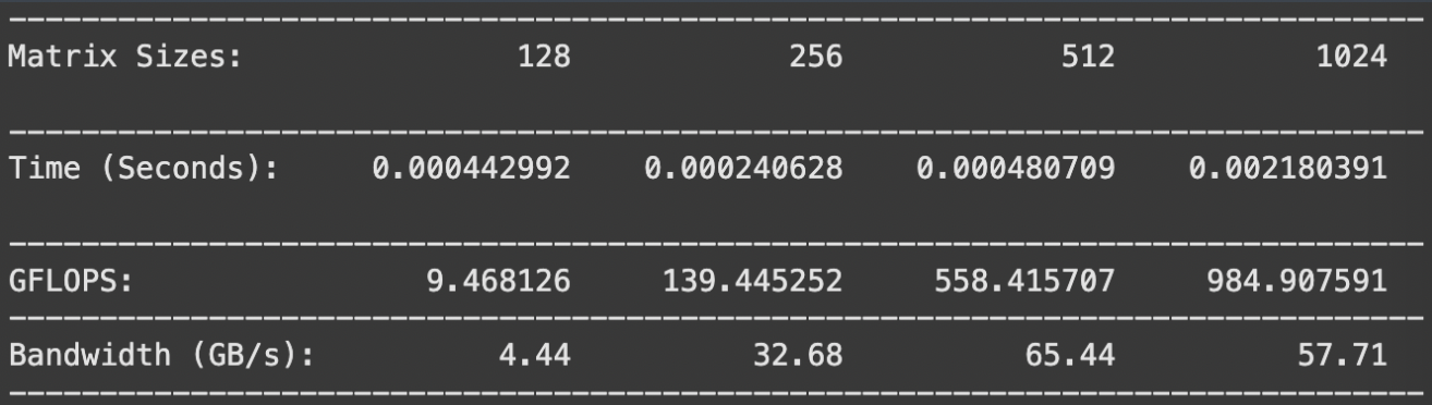
Results
Let’s look at some results for MxM matrices sized 128, 256, 512, and 1024.

Problems with this method
The bandwidth across all sizes looks so much better! AND, our 1024x1024 matrix was able to achieve a 14.28x speedup! GFLOPs look great as well. If everything looks so much better with this slight change in memory access patterns, can we do more to optimize that? The answer is YES!
So far, all we did was optimize how we accessed our elements from global memory. But, we also have the shared memory (SMEM) that is much faster to access. Let’s look at how we can optimize memory access patterns in SMEM with tiling.
GeMM-3: Tiled MatMul
In GeMM-2, we focused on GMEM access. However, even if they are fewer than before, we are still making trips to GMEM which is expensive. This is where tiling comes in. Tiling is a technique where we break our matrices into smaller sub-matrices (tiles) that can fit into shared memory with the assumption that these elements are going to be accessed soon. By loading these tiles into shared memory first, threads can repeatedly access the data much faster than going to global memory each time.
Let’s understand how tiling works in this case with matrix multiplications. Instead of having each thread compute its entire output element by accessing global memory repeatedly, we load small tiles of both input matrices into shared memory. All threads in a block then work with these tiles to compute partial results, synchronize, load the next set of tiles, and continue until they’ve processed all tiles needed for their final output elements.
Code Implementation
#define TILE_WIDTH 32
__global__ void tiled_mat_mul_kernel(float *d_A, float *d_B, float *d_C,
int C_n_rows, int C_n_cols, int A_n_cols)
{
assert(TILE_WIDTH == blockDim.x);
assert(TILE_WIDTH == blockDim.y);
const int b_x = blockIdx.x;
const int b_y = blockIdx.y;
const int t_x = threadIdx.x;
const int t_y = threadIdx.y;
// Initializing row, col and number of tiles
const int row = TILE_WIDTH * b_y + t_y;
const int col = TILE_WIDTH * b_x + t_x;
const int num_tiles = ceil((float)A_n_cols/TILE_WIDTH);
// Shared Memory allocation
__shared__ float sh_A[TILE_WIDTH][TILE_WIDTH];
__shared__ float sh_B[TILE_WIDTH][TILE_WIDTH];
float value = 0;
for (int tile = 0; tile < num_tiles; tile++){
// STEP 1 = loading our tiles onto shared memory
// Matrix A
if ((row < C_n_rows) && ((tile * TILE_WIDTH + t_x) < A_n_cols)){
sh_A[t_y][t_x] = d_A[(row) * A_n_cols + (tile * TILE_WIDTH + t_x)]; }
else { sh_A[t_y][t_x] = 0.0f; }
// Matrix B
if (((tile * TILE_WIDTH + t_y) < A_n_cols) && (col < C_n_cols)){
sh_B[t_y][t_x] = d_B[(tile * TILE_WIDTH + t_y) * C_n_cols + (col)]; }
else { sh_B[t_y][t_x] = 0.0f; }
// sync threads
__syncthreads();
// STEP 2 = calc dot product
for (int k_tile = 0; k_tile < TILE_WIDTH; k_tile++)
value += sh_A[t_y][k_tile] * sh_B[k_tile][t_x];
__syncthreads();
}
// Storing and assigning
if ((row < C_n_rows) && (col < C_n_cols))
d_C[(row)*C_n_cols + (col)] = 1*value + 0*d_C[(row)*C_n_cols + (col)];
}
In the code implementation, we introduce several key changes from our coalesced version. First, we define a TILE_WIDTH which determines the size of our shared memory tiles. We then declare two shared memory arrays sh_A and sh_B that will hold our tiles. The computation is now broken into two phases: loading data into shared memory and performing computations using this shared memory.
When loading tiles, each thread in a block is responsible for loading one element from matrix A and one element from matrix B into shared memory. Notice how we maintain coalesced access during this loading phase — threads still access consecutive memory locations when reading from global memory. We also handle boundary conditions carefully by padding with zeros when we reach matrix edges.

The most interesting part comes in the main computation loop. After loading the tiles and synchronizing all threads (this is crucial to ensure all data is loaded before computation begins), each thread performs its partial dot product computation using only shared memory accesses. This is significantly faster than accessing global memory for each multiplication. After processing one tile, threads synchronize again before loading the next tile.
The beauty of this approach lies in its efficiency: once data is in shared memory, each element can be reused by multiple threads without additional global memory transactions. For example, in a single 32x32 tile from matrix A, each element is used 32 times by different threads computing different output elements. Without tiling, we would need to read this same data from global memory 32 times.
Results
Let’s look at some results for MxM matrices sized 128, 256, 512, and 1024.

Problems with this method
The results show impressive improvements across different matrix sizes. Looking at the bandwidth utilization and GFLOPS metrics, we can see that tiling provides another significant speedup over our coalesced implementation. However, this method isn’t without its challenges. Picking the optimal tile size requires careful consideration of the GPU’s shared memory size and occupancy requirements. Too large a tile size reduces the number of thread blocks that can run concurrently, while too small a tile size doesn’t fully utilize the benefits of shared memory.
GeMM-4: Coarse 1D MatMul
Our tiled implementation showed impressive gains, but we can push the performance even further. The key insight is that each thread is only computing a single element of the output matrix. What if we could make each thread do more work? This is where coarse-grained parallelism comes in. Instead of having each thread compute just one element of matrix C, we’ll have it compute multiple elements in the same column. This reduces the total number of threads needed and allows for better resource utilization.
Code Implementation
#define COARSE_FACTOR 8
#define tiles_Arows 64
#define tiles_Acols 8
#define tiles_Bcols 64
__global__ void coarse1D_mat_mul_kernel(float *d_A, float *d_B, float *d_C,
int C_n_rows, int C_n_cols, int A_n_cols)
{
const int b_x = blockIdx.x;
const int b_y = blockIdx.y;
const int t_x = threadIdx.x;
// 1D -> 2D
const int A_view_ty = t_x / tiles_Acols;
const int A_view_tx = t_x % tiles_Acols;
const int B_view_ty = t_x / tiles_Bcols;
const int B_view_tx = t_x % tiles_Bcols;
// Defining rows and cols for C[row, col] and tiles
const int row = tiles_Arows * b_y + COARSE_FACTOR * (t_x/tiles_Bcols);
const int col = tiles_Bcols * b_x + (t_x % tiles_Bcols);
const int num_tiles = ceil((float)A_n_cols / tiles_Acols);
// Saving in SMEM
__shared__ float sh_A[tiles_Arows][tiles_Acols];
__shared__ float sh_B[tiles_Acols][tiles_Bcols];
float value[COARSE_FACTOR] = {0.0f};
for (int tile = 0; tile < num_tiles; tile++){
if ((b_y * tiles_Arows + A_view_ty < C_n_rows) && ((tile * tiles_Acols + A_view_tx) < A_n_cols)){
sh_A[A_view_ty][A_view_tx] = d_A[(b_y*tiles_Arows + A_view_ty)*A_n_cols + (tile * tiles_Acols + A_view_tx)]; }
else
{ sh_A[A_view_ty][A_view_tx] = 0.0f; }
if (((tile * tiles_Acols + B_view_ty) < A_n_cols) && (b_x * tiles_Bcols + B_view_tx < C_n_cols)){
sh_B[B_view_ty][B_view_tx] = d_B[(tile*tiles_Acols + B_view_ty) * C_n_cols + (b_x * tiles_Bcols + B_view_tx)];
}
else
{ sh_B[B_view_ty][B_view_tx] = 0.0f; }
__syncthreads();
for (int k = 0; k < tiles_Acols; k++)
{
float B_val_register = sh_B[k][B_view_tx];
// Dot product
for (int c = 0; c < COARSE_FACTOR; c++)
value[c] += sh_A[B_view_ty*COARSE_FACTOR+c][k] * B_val_register;
}
__syncthreads();
}
// Storing and assigning
for (int c = 0; c < COARSE_FACTOR; ++c){
if ((row+c < C_n_rows) && (col < C_n_cols)){
d_C[(row+c)*C_n_cols + (col)] = 1*value[c] + 0*d_C[(row+c)*C_n_cols + (col)];
}
}
}
The code is hefty, but it’s worth it I promise!
In this implementation, we introduce the COARSE_FACTOR, which determines how many elements each thread will compute. We’re also changing our approach to tiling by using 1D thread blocks instead of 2D, which requires some clever index manipulation to map our 1D thread structure onto our 2D problem space.
Looking at the code, the first major change is how we handle thread indexing. We’re now converting our 1D thread index (t_x) into appropriate 2D coordinates for both A and B matrix views. The lines A_view_ty = t_x / tiles_Acols and A_view_tx = t_x % tiles_Acols handle this mapping, allowing us to maintain coalesced memory access patterns while working with a 1D thread structure.
The most significant change comes in how each thread processes its work. Instead of a single value variable, we now have an array value[COARSE_FACTOR] where each thread keeps track of multiple partial results. When loading data into shared memory, we maintain our efficient access patterns, but during computation, each thread now processes COARSE_FACTOR elements in the same column of the output matrix.
A subtle but important optimization appears in the main computation loop. Notice how we store B’s value in a register (float B_val_register = sh_B[k][B_view_tx]) before using it in the inner loop. This register caching helps reduce shared memory accesses, as the same B value is used for all COARSE_FACTOR computations within a thread.
Results
Let’s look at some results for MxM matrices sized 128, 256, 512, and 1024.

Problems with this method
Looking at the results, we can see significant improvements over our tiled implementation (GeMM-3). The GFLOPS metrics show substantial gains across all matrix sizes, with particularly impressive scaling for larger matrices. For the 1024x1024 case, we’ve achieved 847 GFLOPS compared to GeMM-3’s 569 GFLOPS — nearly a 1.5x improvement. For the 1024x1024 matrix again, we see a 2.14x speedup! The bandwidth utilization also shows better efficiency, indicating we’re making better use of our memory subsystem.
However, this approach isn’t without its limitations. While 1D coarsening gives us better performance, we’re still not fully utilizing all dimensions of parallelism available to us. The next logical step would be to explore 2D coarsening (GeMM-5), where each thread computes a 2D tile of the output matrix rather than just a column strip. This would allow us to further reduce the number of threads needed and potentially achieve even better resource utilization.
GeMM-5: Coarse 2D MatMul
Building on our success with 1D coarsening, we can push performance even further by extending our coarsening strategy to two dimensions. Instead of having each thread compute multiple elements in a single column, we’ll now have each thread compute a 2D tile of the output matrix. This approach maximizes data reuse and further reduces the total number of threads needed for computation.
The key innovation in this implementation is the introduction of both COARSE_Y and COARSE_X factors, which define the dimensions of the output tile each thread will compute. By having dims of 8x8, each thread is now responsible for computing 64 elements of the output matrix — a significant increase from our previous implementations.
Code Implementation
#define COARSE_X 8
#define COARSE_Y 8
#define tiles_Arows 128
#define tiles_Acols 16
#define tiles_Bcols 128
__global__ void coarse2D_mat_mul_kernel(float *d_A, float *d_B, float *d_C,
int C_n_rows, int C_n_cols, int A_n_cols)
{
// Getting number of threads per block
const int num_threads = tiles_Arows * tiles_Bcols / (COARSE_X * COARSE_Y);
static_assert(num_threads % tiles_Acols == 0);
static_assert(num_threads % tiles_Bcols == 0);
const int b_x = blockIdx.x;
const int b_y = blockIdx.y;
const int t_x = threadIdx.x;
// 1D -> 2D
const int A_view_ty = t_x / tiles_Acols;
const int A_view_tx = t_x % tiles_Acols;
const int B_view_ty = t_x / tiles_Bcols;
const int B_view_tx = t_x % tiles_Bcols;
// Adding strides to load A and B
const int stride_A = num_threads / tiles_Acols;
const int stride_B = num_threads / tiles_Bcols;
// Defining rows and cols for C[row, col] and tiles
const int row = COARSE_Y * (t_x / (tiles_Bcols / COARSE_X));
const int col = COARSE_X * (t_x % (tiles_Bcols / COARSE_X));
const int num_tiles = ceil((float)A_n_cols / tiles_Acols);
// Saving in SMEM
__shared__ float sh_A[tiles_Arows][tiles_Acols];
__shared__ float sh_B[tiles_Acols][tiles_Bcols];
// Mat-Mul Parallelize
float value[COARSE_Y][COARSE_X] = {0.0f};
float register_A[COARSE_X] = {0.0f};
float register_B[COARSE_Y] = {0.0f};
for(int tile = 0; tile < num_tiles; tile++){
for(int load_offset = 0; load_offset < tiles_Arows; load_offset += stride_A){
if (((b_y * tiles_Arows + load_offset + A_view_ty) < C_n_rows) && ((tile * tiles_Acols + A_view_tx) <A_n_cols)){
sh_A[load_offset + A_view_ty][A_view_tx] = d_A[(b_y * tiles_Arows + load_offset + A_view_ty) * A_n_cols + (tile * tiles_Acols + A_view_tx)]; }
else { sh_A[load_offset + A_view_ty][A_view_tx] = 0.0f; }
}
for(int load_offset = 0; load_offset < tiles_Acols; load_offset += stride_B){
if (((tile * tiles_Acols + load_offset + B_view_ty) < A_n_cols) && (b_x * tiles_Bcols + B_view_tx < C_n_cols)) {
sh_B[load_offset + B_view_ty][B_view_tx] = d_B[(tile * tiles_Acols + B_view_ty + load_offset) * C_n_cols + (b_x * tiles_Bcols + B_view_tx)]; }
else { sh_B[load_offset + B_view_ty][B_view_tx] = 0.0f; }
}
__syncthreads();
// per-thread results
for(int k = 0; k < tiles_Acols; ++k){
// into registers
for (int i = 0; i < COARSE_Y; ++i) { register_A[i] = sh_A[row+i][k]; }
for (int i = 0; i < COARSE_X; ++i) { register_B[i] = sh_B[k][col+i]; }
for (int cy = 0; cy < COARSE_Y; ++cy){
for (int cx = 0; cx < COARSE_X; ++cx){
value[cy][cx] += register_A[cy] * register_B[cx];
}
}
}
__syncthreads();
}
// assign calculated value
for (int cy = 0; cy < COARSE_Y; ++cy){
for (int cx = 0; cx < COARSE_X; cx++){
if((b_y * tiles_Arows + row + cy < C_n_rows) && (b_x * tiles_Bcols + col + cx < C_n_cols)){
d_C[(b_y * tiles_Arows + row + cy) * C_n_cols + (b_x * tiles_Bcols + col + cx)] = 1 * value[cy][cx] + 0* d_C[(b_y * tiles_Arows + row + cy) * C_n_cols + (b_x * tiles_Bcols + col + cx)];
}
}
}
}
Looking at the code, we’ve introduced several sophisticated optimizations. First, we’ve added stride parameters (stride_A and stride_B) to handle the loading of data into shared memory more efficiently. Each thread now participates in loading multiple elements, which helps maintain coalesced memory access patterns despite our reduced thread count.
A crucial optimization appears in our register usage. Notice the introduction of register_A and register_B arrays. These register arrays serve as a cache for frequently accessed values from shared memory. When computing the output tile, instead of repeatedly accessing shared memory, we first load the needed values into registers. This dramatically reduces shared memory bandwidth requirements and helps avoid bank conflicts.
The computation kernel shows the heart of our 2D coarsening strategy. The nested loops over COARSE_Y and COARSE_X compute the entire output tile, with all intermediate values stored in the 2D value array. This structure allows for better instruction-level parallelism as the compiler can optimize these tight loops effectively.
Results
Let’s look at some results for MxM matrices sized 128, 256, 512, and 1024.
Problems with this method
Looking at the results, we can see substantial improvements over our 1D coarse implementation. For the 1024x1024 case, we’ve achieved 984 GFLOPS — a significant jump from GeMM-4’s 847 GFLOPS. The bandwidth utilization remains strong, suggesting we’re making efficient use of our memory subsystem while doing more computation per thread.
However, we can still do more. The increased register usage per thread (due to storing larger value arrays and register tiles) can impact occupancy. We’re also pushing the limits of what’s practical in terms of thread coarsening — going much beyond 8x8 tiles would likely start to see diminishing returns due to register pressure and reduced parallelism. The next logical step would be to explore vectorization, where we can leverage the GPU’s vector units to process multiple elements simultaneously. This would allow us to maintain our efficient memory access patterns while potentially reducing register pressure and improving instruction throughput. But that’s a story for GeMM-6, where we’ll see how vectorization can push our performance even further.
GeMM-6: Coarse 2D Vectorized MatMul
Our 2D coarse-grained implementation showed impressive improvements, but we can squeeze in even more performance by leveraging the GPU’s vector processing capabilities. Modern GPUs can load and process multiple elements simultaneously through vectorization. Instead of loading single elements at a time, we can use float4 to load four consecutive elements in a single transaction, significantly reducing memory bandwidth requirements and increasing throughput.
Code Implementation
#define COARSE_X 8
#define COARSE_Y 8
#define tiles_Arows 128
#define tiles_Acols 16
#define tiles_Bcols 128
__global__ void coarse2Dvec_mat_mul_kernel(float *d_A, float *d_B, float *d_C, int C_n_rows, int C_n_cols, int A_n_cols)
{
// Number of threads per block
const int num_threads = tiles_Arows * tiles_Bcols / (COARSE_X*COARSE_Y);
static_assert(num_threads % tiles_Acols == 0);
static_assert(num_threads % tiles_Bcols == 0);
static_assert(tiles_Acols % 4 == 0);
static_assert(tiles_Bcols % 4 == 0);
assert(C_n_rows % 4 == 0);
assert(C_n_cols % 4 == 0);
assert(A_n_cols % 4 == 0);
// Details regarding this thread
const int b_y = blockIdx.y;
const int b_x = blockIdx.x;
const int t_x = threadIdx.x;
// 1D -> 2D while loading A
const int A_view_tx = t_x % (tiles_Acols / 4);
const int B_view_ty = t_x / (tiles_Bcols / 4);
const int B_view_tx = t_x % (tiles_Bcols / 4);
const int A_view_ty = t_x / (tiles_Acols / 4);
// loading A and B
const int stride_A = num_threads/(tiles_Acols / 4);
const int stride_B = num_threads/(tiles_Bcols / 4);
// Working on C[row, col]
const int row = COARSE_Y * (t_x / (tiles_Bcols/COARSE_X));
const int col = COARSE_X * (t_x % (tiles_Bcols/COARSE_X));
const int num_tiles = ceil((float)A_n_cols/tiles_Acols);
// Allocating shared memory
__shared__ float sh_A[tiles_Acols][tiles_Arows];
__shared__ float sh_B[tiles_Acols][tiles_Bcols];
// Parallel mat mul
float value[COARSE_Y][COARSE_X] = {0.0f};
float register_A[COARSE_X] = {0.0f};
float register_B[COARSE_Y] = {0.0f};
for (int tile = 0; tile < num_tiles; tile++)
{
// Load Tiles into shared memory
for (int load_offset = 0; load_offset < tiles_Arows; load_offset+=stride_A)
{
if ((b_y*tiles_Arows + load_offset+A_view_ty < C_n_rows) && (((tile*tiles_Acols+A_view_tx*4)) < A_n_cols))
{
float4 temp_A = reinterpret_cast<float4 *>(&d_A[(b_y*tiles_Arows + load_offset+A_view_ty)*A_n_cols + ((tile*tiles_Acols+A_view_tx*4))])[0];
sh_A[A_view_tx*4+0][load_offset+A_view_ty] = temp_A.x;
sh_A[A_view_tx*4+1][load_offset+A_view_ty] = temp_A.y;
sh_A[A_view_tx*4+2][load_offset+A_view_ty] = temp_A.z;
sh_A[A_view_tx*4+3][load_offset+A_view_ty] = temp_A.w;
}
else
{
sh_A[A_view_tx*4+0][load_offset+A_view_ty] = 0.0f;
sh_A[A_view_tx*4+1][load_offset+A_view_ty] = 0.0f;
sh_A[A_view_tx*4+2][load_offset+A_view_ty] = 0.0f;
sh_A[A_view_tx*4+3][load_offset+A_view_ty] = 0.0f;
}
}
for (int load_offset = 0; load_offset < tiles_Acols; load_offset+=stride_B)
{
if (((tile*tiles_Acols + B_view_ty+load_offset) < A_n_cols) && (((b_x*tiles_Bcols + B_view_tx*4)) < C_n_cols))
{
float4 temp_B = reinterpret_cast<float4 *>(&d_B[(tile*tiles_Acols + B_view_ty+load_offset)*C_n_cols + ((b_x*tiles_Bcols + B_view_tx*4))])[0];
sh_B[B_view_ty+load_offset][B_view_tx*4+0] = temp_B.x;
sh_B[B_view_ty+load_offset][B_view_tx*4+1] = temp_B.y;
sh_B[B_view_ty+load_offset][B_view_tx*4+2] = temp_B.z;
sh_B[B_view_ty+load_offset][B_view_tx*4+3] = temp_B.w;
}
else
{
sh_B[B_view_ty+load_offset][B_view_tx*4+0] = 0.0f;
sh_B[B_view_ty+load_offset][B_view_tx*4+1] = 0.0f;
sh_B[B_view_ty+load_offset][B_view_tx*4+2] = 0.0f;
sh_B[B_view_ty+load_offset][B_view_tx*4+3] = 0.0f;
}
}
__syncthreads();
// calculate per-thread results
for (int k = 0; k < tiles_Acols; ++k)
{
// block into registers
for (int i = 0; i < COARSE_Y; ++i)
register_A[i] = sh_A[k][row+i];
for (int i = 0; i < COARSE_X; ++i)
register_B[i] = sh_B[k][col+i];
for (int cy = 0; cy < COARSE_Y; ++cy)
{
for (int cx = 0; cx < COARSE_X; ++cx)
value[cy][cx] += register_A[cy] * register_B[cx];
}
}
__syncthreads();
}
// Assigning calculated value
for (int cy = 0; cy < COARSE_Y; ++cy)
{
for (int cx = 0; cx < COARSE_X; cx++)
{
if ((b_y*tiles_Arows+row+cy < C_n_rows) && (b_x*tiles_Bcols+col+cx < C_n_cols))
d_C[(b_y*tiles_Arows+row+cy)*C_n_cols + (b_x*tiles_Bcols+col+cx)] = 1*value[cy][cx] + 0*d_C[(b_y*tiles_Arows+row+cy)*C_n_cols + (b_x*tiles_Bcols+col+cx)];
}
}
}
Looking at the code, the most significant changes appear in our memory loading patterns. We’re still using the same 2D coarsening strategy where each thread computes an 8x8 tile of the output matrix, but we’ve completely restructured how data is loaded into shared memory. The introduction of float4 and reinterpret_cast allows us to load four consecutive elements in a single operation.
A key optimization appears in our memory indexing calculations. Notice how we’ve adjusted our view indices to account for vectorized loading: A_view_tx = t_x % (tiles_Acols / 4) and B_view_tx = t_x % (tiles_Bcols / 4). This ensures our vectorized loads maintain proper alignment and coalescing. The division by 4 in these calculations directly reflects our use of float4 vectors.
The loading of matrices into shared memory showcases the power of vectorization. When loading matrix A, we use float4 to grab four consecutive elements and then unpack them into shared memory:
float4 temp_A = reinterpret_cast<float4 *>(&d_A[...])[0];
sh_A[A_view_tx*4+0][load_offset+A_view_ty] = temp_A.x;
sh_A[A_view_tx*4+1][load_offset+A_view_ty] = temp_A.y;
sh_A[A_view_tx*4+2][load_offset+A_view_ty] = temp_A.z;
sh_A[A_view_tx*4+3][load_offset+A_view_ty] = temp_A.w;
This vectorized loading requires careful attention to alignment, which we enforce through static assertions. Notice the checks ensuring tiles_Acols and tiles_Bcols are multiples of 4, along with runtime assertions for matrix dimensions. These requirements ensure our vectorized operations work correctly and efficiently.
Interestingly, while the loading phase has been heavily modified for vectorization, the computation phase remains similar to our 2D coarse implementation. This highlights a key principle in GPU optimization: often, the biggest gains come from optimizing memory access patterns rather than computation patterns.
Results
Let’s look at some results for MxM matrices sized 128, 256, 512, and 1024.

Voila! This looks so much better than what we started with!! Although, I am not sure what is going on with our 128x128 matrix (yikes!). I believe we could have used better coarse factors and optimization settings to better suit a 128x128 matrix. However, my focus for this post was on 1024x1024. Let’s compare those gains!
FINAL RESULTS

Looking at our journey from GeMM-1 to GeMM-6, the progression in performance is remarkable. Let’s analyze the results for 1024x1024 matrices across all implementations:
Our baseline GeMM-1 achieved merely 22.27 GFLOPS with a bandwidth of 1.31 GB/s. The introduction of coalescing in GeMM-2 gave us our most dramatic single improvement, jumping to 318.12 GFLOPS — a 14.28x speedup. Tiling in GeMM-3 further improved performance to 395.52 GFLOPS, while 1D coarsening in GeMM-4 nearly doubled this to 847.04 GFLOPS.
The transition to 2D coarsening in GeMM-5 pushed us to 984.91 GFLOPS, and finally, our vectorized implementation in GeMM-6 achieved 1348.33 GFLOPS with a bandwidth of 79.00 GB/s. This represents a cumulative speedup of 60.56x over our initial implementation.
What’s particularly interesting is the scaling pattern. The largest jumps came from our initial optimizations (coalescing and initial tiling), but each subsequent optimization still provided meaningful improvements. This demonstrates the compound effect of these optimizations — each one building on the foundations laid by previous improvements.
The final bandwidth utilization of 79.00 GB/s suggests we’re making excellent use of the memory subsystem, while the GFLOPS metric shows we’re achieving high computational efficiency. This implementation represents a careful balance of all the optimization techniques we’ve explored: coalesced memory access, efficient use of shared memory, thread coarsening, and vectorized loading.
I hope this was helpful!