Low-Precision Arithmetic in ML Systems
Have you ever wondered how modern AI systems handle billions of calculations without melting your computer? The secret sauce lies in something called low-precision arithmetic. Let’s dive into what this means and why it matters.
Have you ever wondered how modern AI systems handle billions of calculations without melting your computer? The secret sauce lies in something called low-precision arithmetic. Let’s dive into what this means and why it matters.
What is Numerical Precision?
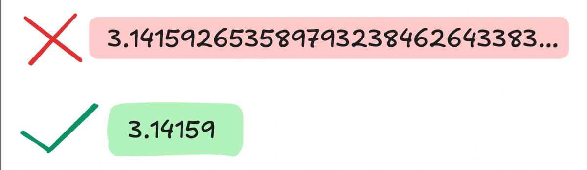
Before we jump into the low-precision world, let’s understand what numerical precision means in computing. Think of it like writing numbers like pi: you can write 3.14159265359 (high precision) or just 3.14 (lower precision). In computers, we store numbers using bits, and fewer bits means lower precision but faster calculations and less memory use.
I remember my math teacher often told us to round pi up to 4 decimal points because we didn’t need too much precision for our calculations to be accurate for our job at hand. Similarly, our ML workloads don’t benefit a lot from precision during certain phases of the model. For example, training our model would definitely require more precision than at inference. This is why we need Low Precision Arithmetic — to figure out when we can benefit from lowering precision without compromising on accuracy.
Common Precision Formats in ML
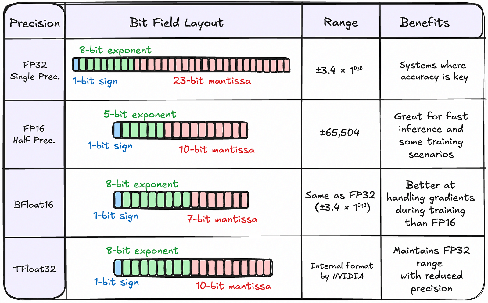
Figure 2. definitely gives a more comprehensive overview of our precision types. For clarity, bit field representation is commonly used to illustrate the structure and organization of floating-point formats, showing how the total bits are partitioned into different components and their respective positions within the binary representation. Range in floating-point numbers refers to the interval between the smallest and largest numbers that can be represented in that format. For example, in FP32, the range is approximately ±3.4 × 1⁰³⁸, meaning it can represent numbers from about -3.4 × 1⁰³⁸ to +3.4 × 1⁰³⁸, but numbers outside this range will cause overflow or underflow.
Let’s talk about their quirks very briefly…
FP32 (32-bit Floating Point)
This is the traditional workhorse of machine learning. Think of it as the comfortable family sedan — reliable, good at everything, but not the most efficient choice for every situation.
FP16 (16-bit Floating Point)
Half-precision floating point is like a sporty compact car — lighter and more efficient, but with some limitations.
BF16 (Brain Floating Point)
BF16 is like a clever hybrid vehicle — it combines the best of both worlds. It’s specifically designed for machine learning.
TF32 (Tensor Float 32)
NVIDIA’s specialized format that’s like a tuned-up version of FP32, optimized for ML workloads. It maintains FP32 range with reduced precision.
Impact on Hardware and Software
Benefits
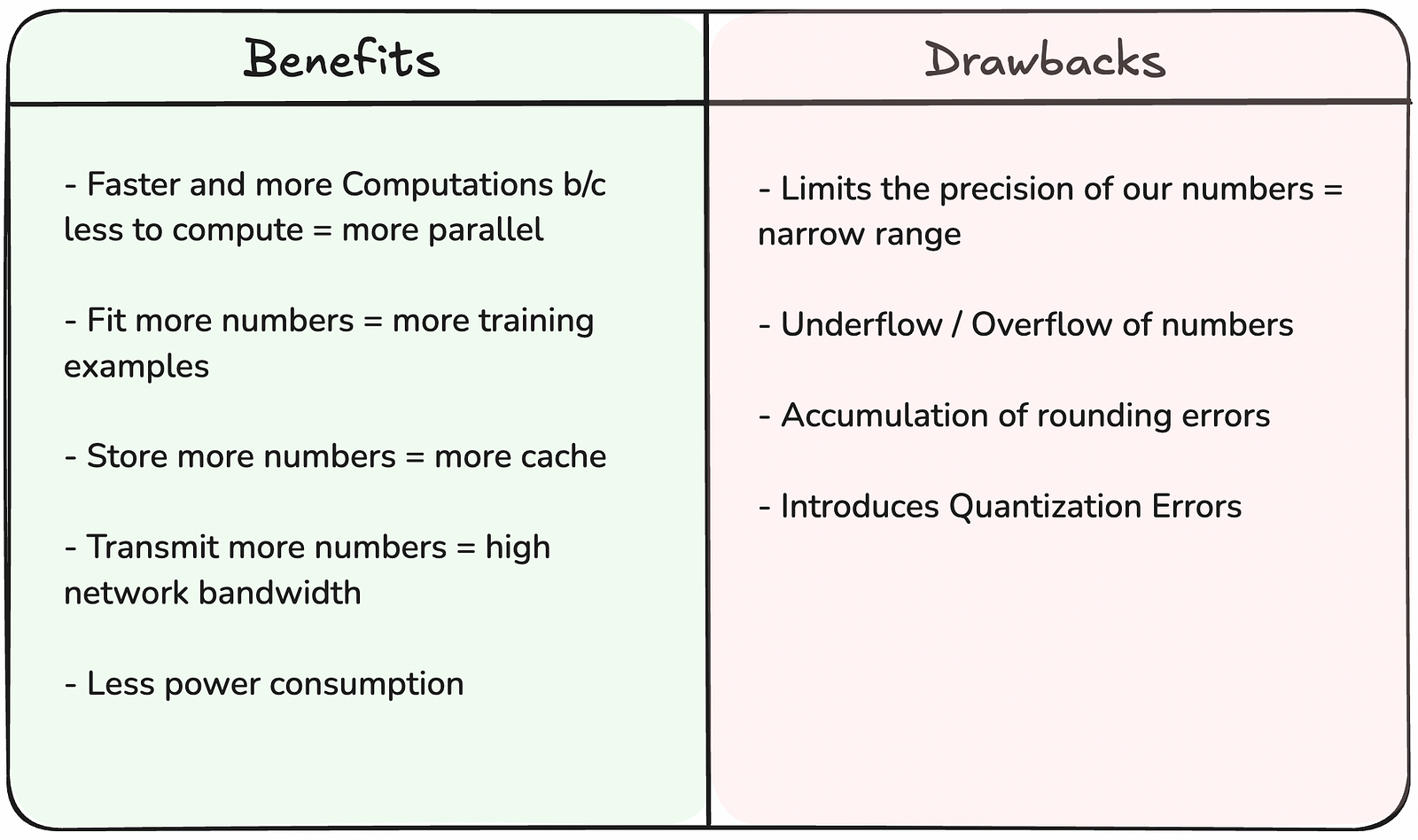
The adoption of low-precision arithmetic brings substantial benefits to both hardware and software aspects of machine learning systems. We can think of these benefits in four folds — storage, data, power, and communication. On the hardware side, the impact is immediately noticeable in memory bandwidth utilization. When using FP16, systems can effectively double their memory bandwidth, allowing for more efficient and easier data movement between memory and compute units. This improvement extends to cache utilization, where more data can fit into the same cache space, reducing expensive memory accesses and improving overall system performance.
The computational benefits are equally impressive. Matrix multiplications, which form the backbone of many ML operations, can run up to twice as fast with FP16 compared to FP32. When using specialized hardware designed for low-precision operations, these speedups can reach up to 8x. This acceleration comes with an added bonus of reduced power consumption per operation, making low-precision arithmetic an environmentally friendly and cost efficient choice for large-scale ML deployments.
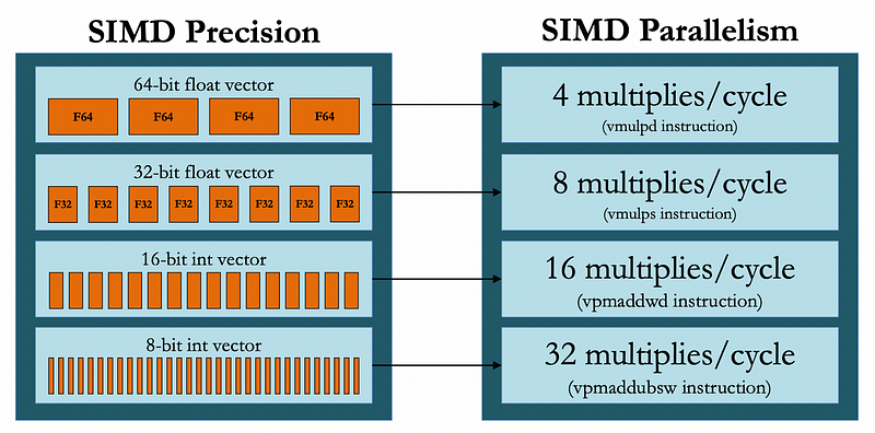
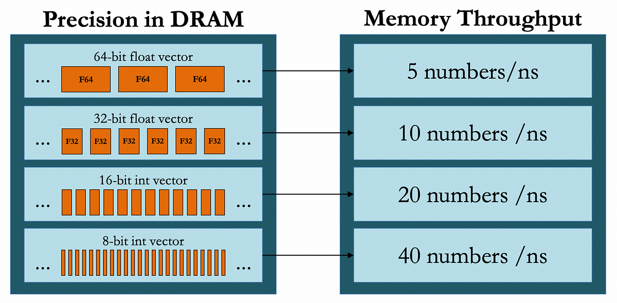
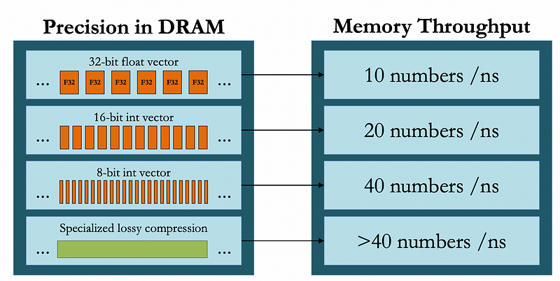
Figure 3. Compute, Memory, and Communication Benefits for the Precision Types | Source: Cornell Lecture 21
Drawbacks
From a software perspective, implementing low-precision arithmetic requires careful consideration of numerical stability. While FP16 can significantly speed up computations, it comes with risks of overflow and underflow that need to be managed. Modern ML frameworks address this through techniques like loss scaling during training and gradient accumulation in higher precision.
In our computations, when calculations depend on the results of previous calculations (inter-dependent computations), rounding errors can compound and grow larger over time. This is known as accumulation of rounding errors. This is similar to a game of telephone — each time a number is rounded and passed to the next computation, the small error from rounding gets added to new rounding errors, potentially leading to significant deviations from the true result after many steps. This issue is particularly relevant in deep neural networks where errors from earlier layers can propagate and amplify through the network, potentially affecting model convergence or accuracy.
Another drawback to this in our ML Systems is the introduction to Quantization Errors. Quantization refers to the process of converting a number from a higher precision format to a lower precision. We usually
The good news is that when implemented correctly, the impact on final model accuracy is usually minimal, though some architectures may require additional tuning to maintain their performance.
Applying it in our ML Workloads + Impact
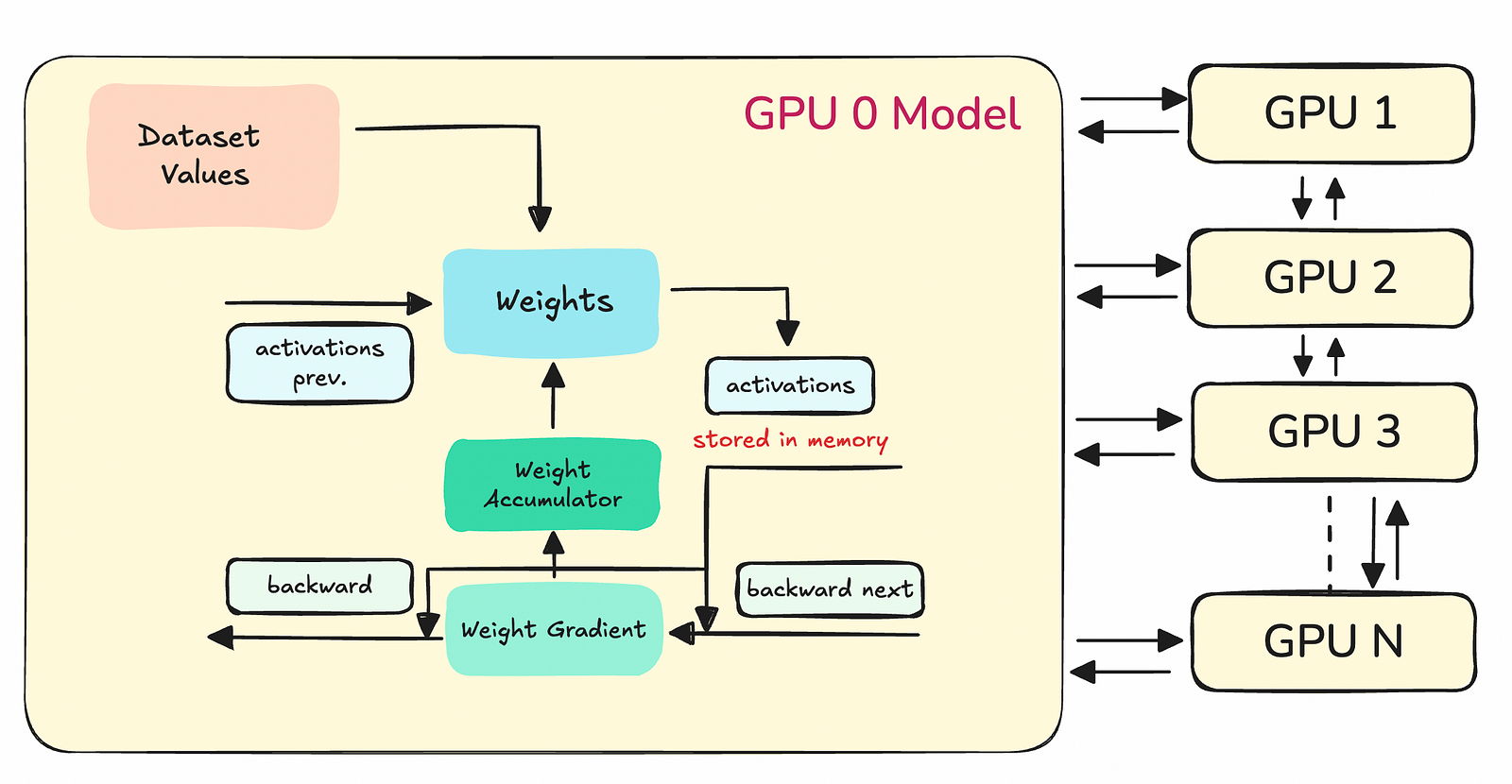
Let’s recall the setup of our typical Deep Neural Network (DNN) models to understand how precision is crucial during training. When we talk about the training of DNNs, it involves several kinds of numerical values, each playing a different role in the learning process. These values include weights, activations from the current and previous layers, gradients, and more. For efficiency, each of these signals forms a class of numbers, and we often assign a specific precision to each class. Notably, different classes can have varying levels of precision based on their role and impact on the training dynamics.
We typically have 4 number classes that can benefit from precision-manipulation. Each class of numbers has a distinct role:
- Dataset Numbers handle values from our dataset that has been cleaned, handled, and tokenized to be fed into our DNN model.
- Activation numbers and backward pass numbers help in calculating the outputs from layers and the error propagation backwards through the network.
- Weight accumulators and linear layer accumulators are vital in updating the weights and hence, the learning aspect of the network.
- Communication numbers help us transmit and accumulate values from other GPUs in a distributed system. These are values that need to be communicated between devices and host during the synchronization steps.
Quantizing these 4 classes of numbers have huge memory and statistical impacts which often work against each other. Let’s discuss those:
- Dataset numbers: Handling large datasets efficiently by quantizing these numbers, thus improving memory capacity and training example throughput. However, quantizing these values often means that we are solving a different problem altogether because our data is fundamentally represented different. Also, we often don’t realize the impact of precision at this stage.
- Model/weight numbers: By quantizing these, we enhance cache capacity and reduce the computational overhead. However, this also adds noise to each gradient step which dissolves the representation of our solution.
- Gradient numbers: These are crucial for backpropagation, and quantizing them can significantly cut down computational costs. However, if not handled properly, this can introduce errors in calculations — especially through accumulation of rounding errors.
- Communication numbers: In distributed training environments, quantizing these numbers reduces the load on inter-worker memory bandwidth, which is often a bottleneck during synchronization. However, errors during quantization can result in the models to diverge from its local workers causing slow convergence across devices.
Strategies to resolve some issues
Reducing precision introduces noise primarily in the form of round-off errors. There are generally two approaches to manage this rounding:
- Biased rounding: This method rounds to the nearest number, which might introduce a systematic error.
- Unbiased rounding: This strategy involves rounding randomly, which helps in averaging out the errors over many iterations, thus mitigating some negative impacts.
Let’s discuss some more techniques like this….
Techniques for Preserving Accuracy in Low-Precision Arithmetic
When working with low-precision formats, several sophisticated techniques have been developed to maintain computational accuracy while still benefiting from the efficiency gains. Training stability becomes particularly important when working with lower precision formats. Regular monitoring for NaN values, keeping track of loss scaling statistics, and checking gradient norms should become part of your training routine. Additionally, different layers in your model may benefit from different precision levels. A common pattern is to keep the first and last layers in higher precision while using lower precision for middle layers, as these layers are often more tolerant of reduced precision.
- Loss scaling is perhaps the most fundamental of these techniques — it involves multiplying the loss by a large factor before backpropagation and then dividing the gradients by the same factor. This helps prevent gradients from becoming too small for low-precision representations to handle effectively.
- Gradient accumulation in higher precision has emerged as another crucial strategy. While the forward pass and gradient computations might use low precision (like FP16), gradients are accumulated in FP32. This prevents the accumulation of rounding errors during the optimization process while still maintaining most of the performance benefits of low-precision arithmetic.
- Mixed-precision training takes this concept further by dynamically selecting precision levels for different operations. This is definitely the most popular and prevalent technique to preserve accuracy. Critical numerical operations that are sensitive to precision are performed in FP32, while bulk matrix multiplications that can tolerate lower precision are done in FP16 or BF16. Modern frameworks handle this switching automatically, optimizing the balance between performance and accuracy.
- Stochastic rounding has proven particularly effective in very low precision scenarios. Instead of always rounding to the nearest representable number, this technique occasionally rounds up or down based on the proximity to the nearest values. This introduces a small amount of noise but ensures unbiased estimates over time, often leading to better training dynamics.
These techniques, when properly implemented, allow us to push the boundaries of low-precision arithmetic while maintaining model accuracy. The key is understanding which techniques to apply based on your specific use case and computational requirements.
Practical Implementation
Implementing low-precision arithmetic in modern ML frameworks has been made surprisingly straightforward with current tools for ML workloads — let’s look at PyTorch and CUDA briefly. In PyTorch, automatic mixed precision training, implemented as torch.cuda.amp, can be enabled with just a few lines of code:
# Enable automatic mixed precision
from torch.cuda.amp import autocast, GradScaler
# Create gradient scaler
scaler = GradScaler()
# Training loop
with autocast():
outputs = model(inputs)
loss = criterion(outputs, labels)
# Scale loss and do backward pass
scaler.scale(loss).backward()
scaler.step(optimizer)
scaler.update()
For CUDA-level optimizations, enabling TF32 on Ampere GPUs is equally simple:
// Enable TF32 (on Ampere GPUs)
cudaDeviceSetAttribute(cudaDevAttrTensorFloatPrecision,
CUDA_TENSOR_FLOAT32_PRECEDENCE);
Choosing the Right Precision
The choice of precision format should be guided by your specific use case and requirements. FP32 remains the go-to choice for initial development and debugging, where stability and ease of development take precedence over performance optimization. For production inference and well-tested training pipelines, FP16 offers an excellent balance of performance and accuracy. When FP16 proves unstable, particularly in training large models, BF16 provides a robust alternative with its extended dynamic range. TF32, available on modern NVIDIA GPUs, offers an automatic acceleration path that requires minimal code changes.
This is a very high overview of how to choose the right precision. The decision, ultimately, falls on your workload’s hardware and software configurations.
Real-World Impact and Conclusion
The impact of low-precision arithmetic in real-world ML applications cannot be overstated. Organizations implementing these techniques typically see training times reduced by 2–3x, memory usage cut by up to 75%, and significant reductions in energy consumption. These improvements not only accelerate development cycles but also make it possible to train larger, more complex models that would be impractical with traditional FP32 arithmetic.
Low-precision arithmetic has emerged as a fundamental technique in modern ML systems, offering a carefully balanced approach to computational efficiency and numerical accuracy. While it requires attention to implementation details, the benefits in terms of speed, memory usage, and energy efficiency make it an essential tool for ML practitioners. Remember that success with low-precision arithmetic isn’t about always using the lowest possible precision, but about choosing the right precision for each task. Start with mixed precision training, monitor your results carefully, and adjust based on your specific needs and constraints.